
An Exercise in Unsupervised Learning
Python, Statistics ·Introduction
In this write-up, we shall take a look at the data set “Do we still need gyms?” found on Kaggle. The authors consider the notion that gyms are no longer needed if the gains obtained from going to the gym can be replaced by medicine. While we are not going to directly answer the question posed by the authors, we are going to be making an assessment of the data. The goal is to find participants that are grouped together in some manner and explain the methods used to find said groups.
In what follows, we conduct exploratory data analysis (EDA) and use two unsupervised learning techniques to find subgroups or clusters within the data: \(K\)-Means Clustering and Density-Based Spatial Clustering of Applications with Noise (DBSCAN).
Why are these called unsupervised? Unsupervised learning algorithms operate without any guidance from a known “target” value. That is, the “target” value would be a known feature of the data and the algorithm would refer to this “target” to validate its process of “learning” about the provided data. Since no “target” is present, unsupervised learning algorithms perform a series of steps to partition the data according to a set of rules or conditions without a validation step.
The authors built their data set with five characteristics on \(1000\) participants. Three characteristics were recorded before and after any medicine was administered to the individuals. In our exploration, we consider the weight (Kg) and the medicine taken (“\(1\)”, “\(2\)”, and/or “\(3\)”).
Describing The Algorithms
We note that the algorithms will operate in Euclidean space, where the horizontal axis represents one feature of interest and the vertical axis represents the other feature of interest.
\(K\)-Means Algorithm
This algorithm offers a simple and effective approach to find subgroups. Aside from the data, the only input to the algorithm is \(K\), the number of clusters one expects to see from the data. Every point in the data set will be assigned to one of the clusters.
The algorithm uses a metric, called the within-cluster variation, as a way to assign points to a cluster. The within-cluster variation is denoted \(W(C_{i})\), where \(C_{i}\) is the \(i\)th cluster (up to and including \(K\)). The authors of An Introduction to Statistical Learning note that \(W\) is most commonly defined in terms of squared Euclidean distances. In other words, the metric is constructed by the squared differences between points in a cluster. This is an optimization problem because we want to make \(W\) as small as possible. Mathematically speaking, the algorithm solves
\[\begin{equation*} \underset{C_{1}, \dots, C_{K}}{\text{minimize}} \left\{ \sum_{i = 1}^{K} W(C_{i}) \right\} \text{.} \end{equation*}\]It turns out that W can be re-written in terms of the means of the features in question. Select the points that belong to the \(i\)th cluster. Then, for each feature, take an average of the selected points. The resulting averages form the centroid of the \(i\)th cluster. With that in mind, the \(K\)-Means algorithm is performed in two steps:
- Step 1: randomly assign an observation to one of the \(K\) clusters
- Step 2: repeat the following steps until cluster assignment stops changing
- a. calculate the centroid of each cluster
- b. assign each observation to the closest centroid
In Step \(2\), cluster assignment stops changing when \(W\) stops decreasing. We obtain a local optimum.
DBSCAN Algorithm
This algorithm is more elaborate and uses the idea of “closeness” or “density” to detect subgroups. To illustrate “closeness”, imagine that a circle around a point \(p\) indicates a level of visibility. If we are able to see other points within a fixed radius, then we say that those points are in the neighborhood around the point \(p\). Let us call the radius of the circle “eps”.
One might suspect that all neighborhoods should contain a minimum number of points, called “minpts”. However, this is unlikely because some points’ neighborhoods will contain less points than others. To get around this, the “minpts” restriction is somewhat relaxed.
Three terms are defined in “A Density-Based Algorithm for Discovering Clusters in Large Spatial Databases with Noise” to cement the idea of “closeness”: directly density-reachable, density-reachable, and density-connected. We restate the definition of the first term and briefly mention the other two definitions.
Definition \(\mathbf{1}\) (Directly Density-Reachable). A point \(p\) is directly density-reachable from a point \(q\) with respect to “eps” and “minpts” if
- \(p\) is in the neighborhood around \(q\)
- the neighborhood contains more points than “minpts” points
It follows that a point \(p\) is density-reachable from a point \(r\) if we can reach \(p\) through a chain of directly density-reachable points. Likewise, points \(p\) and \(q\) are density-connected if there is a point \(o\) such that points \(p\) and \(q\) are density-reachable from point \(o\).
As a result, the DBSCAN algorithm is performed by starting at an arbitrary point \(p\) in the data set and getting all of the points that are density-reachable from point \(p\). The retrieved points are assigned to a cluster, say cluster “\(1\)”. If a point is encountered that is unclassified, meaning it does not yet belong to a cluster, then it is labeled to be part of the current cluster value. Some points are labeled as noise because it does not fit Definition \(1\). The algorithm continues with the next point in the data set until all points have been visited.
Exploring The Data
As part of the exploration, we can obtain summary statistics for the numerical features of the data. Now, let us plot the feature “KgBefore” against the feature “KgAfter”.
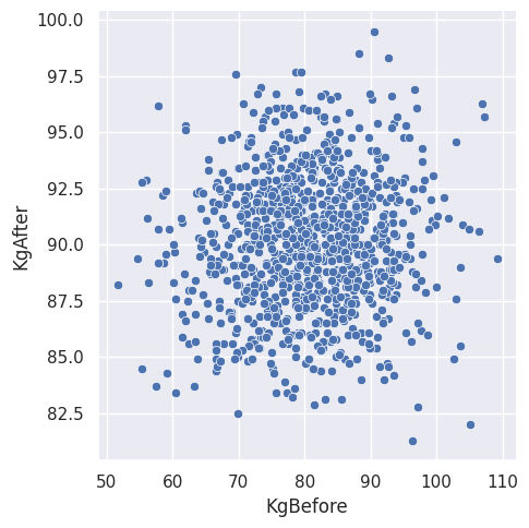
Figure \(1\). The participants’ weight before and after any medicine is administered.
We can see that the points are closely packed. It might be interesting to limit the number of observations that are shown in the plot. For that reason, let us partition the data set as follows: assign the observations of the participants a label based on which medicine was given. Therefore, participants that did not take any medicine will have a label called “\(000\)”. Participants that took medicine \(1\) will have a label called “\(100\)”, and so on. Labeling the data in this manner can be achieved in a few lines of code.
By taking the counts of each partition, we find something worth pointing out: there are individuals that record having side effects, despite not taking any of the medicines. We suppose that it is possible that these individuals were given a placebo. However, we cannot be certain because of the unknown nature on how the data was collected. Everyone else has a tenable reason for reporting side effects given they took one of three distinct medicines or a combination thereof. We can also see that there are some individuals that report having no side effects despite taking all three medicines. One wonders how these medicines affected these participants so that they would not get any side effects.
As we explore the data, here is a box plot of the weight ratios (after over before) for each partition we created before. We can see that the means of the box plots hover around the value of \(1.1\). We also see possible outliers from each partition.
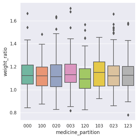
Figure \(2\). Boxplot summary statistics by partition.
We hope that the observation are going to be separated so that the subgroups are clearer to identify, both visually and algorithmically. Let us execute the algorithms and discuss what we find.
Classifying The Clusters
\(K\)-Means Algorithm
The following two graphs show the results of executing the \(K\)-Means algorithm with \(K = 3\). The first plot is for the partition labeled “\(000\)”, the partition where no one took any medicine. The second plot is for the partition labeled “\(123\)”, the partition where participants took all three medicines.
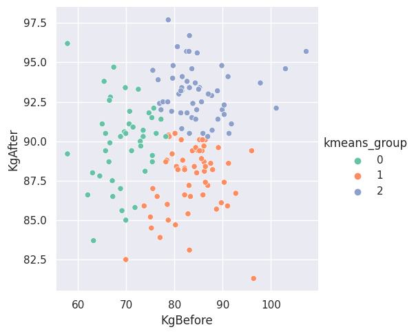
Figure \(3\). Subgroups found by the \(K\)-Means algorithm for the participants that did not take any medicine.
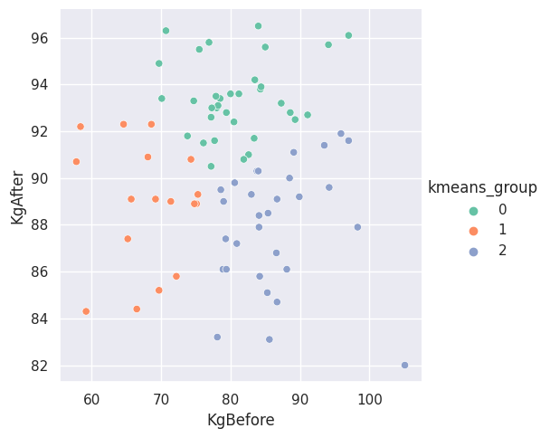
Figure \(4\). Subgroups found by the K-Means algorithm for the participants that took all three medicines.
What are the subgroups saying about the data in these partitions? It is difficult to say. We pondered with the idea that one of the other features could help provide some insight. If we were to inflate the points based on a second feature of the data set, we could question the significance of the points that appear more inflated within one of the groups. It is possible that the inflated points also helps us explain similarities or differences between the subgroups and what it means to be in one subgroups than another subgroup.
DBSCAN Algorithm
Now, we present the DBSCAN algorithm’s execution in the figure below.
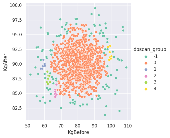
Figure \(5\). Subgroups found by the DBSCAN algorithm for the entire set of participants.
The algorithm found several groups of various sizes. We can see the biggest group stems from the middle of the scatterplot, while smaller groups surround the bigger group. There are also points labeled to be noise, which are shown in the legend with a label of “-\(1\)”. The question is: what can we infer based on the subgroups obtained?
One thing we can question is the significance of the neighborhood radius. Perhaps the radius indicates a level of medicine similarity between participants within the same subgroup (and possibly within different subgroups). That is, individuals in the same group might have similar doses of medicines that was administered. We cannot say for certain and other factors might play a role.
What about those outside the subgroups? We suppose there might be plenty of interpretations for these individuals. For example, much like outliers that require some level of attention, the noise points could be removed or adjusted. In fact, what connection, if any, is there between these points with no subgroup and the outliers in the weight ratios plot?
Conclusion
This write-up summarized the \(K\)-Means and DBSCAN algorithms to finding subgroups or clusters within the data set “Do we still need gyms?”. These techniques are called unsupervised because they execute steps to find an optimum subgroup without a “target” feature. The only input to the cluster techniques are the data and their own specific parameters.
We opted to filter out specific participants from the data set to then build subgroups using the \(K\)-Means algorithm. This allowed us to question any similarities or differences between members of distinct subgroups. In contrast, we fed the unfiltered data set into the DBSCAN algorithm to construct the subgroups. With the found subgroups, we can think about the significance of the neighborhood radius, as well as the points labeled as noise.
We hope this summary of two unsupervised learning algorithms provides a stepping stone for further reading and exploration. We encourage the reader to visit the references for this write-up for in-depth explanations of the algorithms and to continue to think about the questions we asked in previous sections. A Kaggle Notebook is available with the code used to generate the figures.
References
- Martin Ester et al. “A density-based algorithm for discovering clusters in large spatial databases with noise”. In \(96.34\) \((1996)\), pp. \(226-231\).
- Gareth James et al. An introduction to statistical learning. Vol. \(112\). Springer, \(2013\).